RNN

Standard architectures like cnn and mlp process independent inputs conveniently. There is an assumption that each input is quite independent of the other inputs, i.e. they are independent and indentically distributed (i.i.d). If you feed a picture of cat today and a picture of dog tomorrow, the model treats each as isolated events.

This does not hold well with sequential tasks like time series data or language. Here context dictates the output just as much as the immediate input. For example ‘bank’ has different meanings when used as in ‘river bank’ and ‘institutional bank’.

It is quite difficult to determine the meaning of the word for lack of context. one to many mappings could only made less ambiguous with context.

language, audio, timeseries all are context-dependent.

Beyond context incompatibility, traditional nns also happen to have a structural constraint which having fixed length inputs (X belongs to R of n). They usually take a fixed size vector X. A cnn takes a fixed size pixel grid and mlps require a fixed size feature vector. But a sequences (sentences, audio frames) come with variable lengths T.

How can we introduce memory in nn?

Instead of throwing away previous steps output, if we can pass it along the current input as a ‘state vector’. Here we’ve loosely come around the concept of rnns. Rnn is a network loop that passes a persistent memory vector ht down the timeline with the immediate input.

As quoted in Goodfellow et al; a rnn fundamentally is an unfolded computational graph across time.

To make ‘unfolding’ a lot clearer, we take the temporal loop and construct it into a standard Directed Acyclic Graph (DAG). The fundamental necessity for backpropagation to work is an explicit path from input to output.

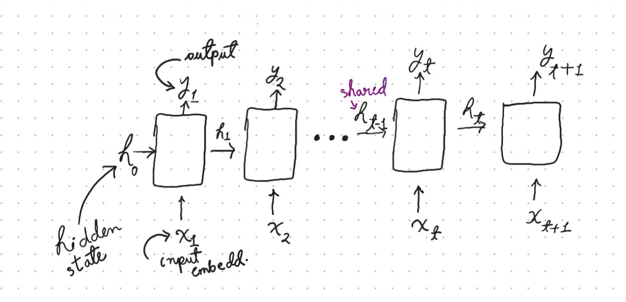
The parameter $h_t$ is the model’s running summary of everything it has seen so far. Because $h_t$ is a function of the current input $x_t$ and the previous hidden state $h_{t-1}$, expanding it recursively reveals that $h_1$ encodes $x_1$, $h_2$ encodes $(x_1, x_2)$, and $h_t$ encodes the entire sequence history $(x_1, x_2, \dots, x_t)$.

In flight, at each time step, the rnn takes in an input $x_t$ and previous hidden state $h_{t-1}$, combines them through their respective shared weights, and runs them through a non-linearity:

$$h_t = \tanh(W_{hh} h_{t-1} + W_{xh} x_t + b_h)$$

This new hidden state $h_t$ is passed forward to the next iteration step. If we want a prediction at step $t$, we pass $h_t$ through an output layer:

$$\hat{y}_t = \text{softmax}(W_{hy} h_t + b_y)$$

One of these steps is considered as one time step.

Sometimes it is called a layer across time too though this is to be noted that it is not literally a separate layer as each iteration uses the same weights. This is one of the defining features of rnn, in standard textbooks it is also called parameter sharing or weight sharing.

Looking backward, without weight sharing, the parameter count would scale linearly with the input and generalization of seq length beyond what was seen during training is also missed out on.

Three questions:

1. how do we compute total loss across a seq? To train an rnn, we must compute loss at each time step t (for example cross entropy loss between prediction y’t and gt yt). Total loss for an entire sequence of length T is simply the sum of losses that happened across all time steps.

$$L = \sum_{t=1}^{T} L_t$$

2. How do we compute the gradient for a weight matrix ($W_{hh}$) that is shared across all time steps? And because $W_{hh}$ is shared across all time steps, updating it requires it contribution to loss at each time step t:

$$\frac{\partial L}{\partial W_{hh}} = \sum_{t=1}^{T} \frac{\partial L_t}{\partial W_{hh}}$$

3. What happens when we backpropagate across long sequences over time? Chain rule across time: Look at a single loss term $L_t$ at step $t$. Since $h_t$ depends on $h_{t-1}$, which depends on $h_{t-2}$, all the way back to $h_0$, applying the chain rule to $\frac{\partial L_t}{\partial W_{hh}}$ yields:

$$\frac{\partial L_t}{\partial W_{hh}} = \sum_{k=1}^{t} \frac{\partial L_t}{\partial h_t} \cdot \frac{\partial h_t}{\partial h_k} \cdot \frac{\partial^+ h_k}{\partial W_{hh}}$$

Focus on that middle term, $\frac{\partial h_t}{\partial h_k}$. It represents the gradient flowing backward through hidden states from step $t$ down to step $k$. By the chain rule, it expands into a product of Jacobians:

$$\frac{\partial h_t}{\partial h_k} = \prod_{j=k+1}^{t} \frac{\partial h_j}{\partial h_{j-1}}$$

Hitting the Mathematical Wall

Differentiating $h_j = \tanh(W_{hh} h_{j-1} + W_{xh} x_j + b_h)$ with respect to $h_{j-1}$ gives:

$$\frac{\partial h_j}{\partial h_{j-1}} = \text{diag}(1 - \tanh^2(\dots)) \cdot W_{hh}$$

When backpropagating across a long sequence (say $T = 50$), you multiply $W_{hh}$ by itself 50 times:Vanishing Gradient: If the largest singular value of $W_{hh}$ is less than 1 (or because $\tanh'$ derivatives are $\le 1$), multiplying these matrices repeatedly causes the gradient to decay exponentially toward zero. Steps far in the past receive zero gradient update. The model forgets long-term context.Exploding Gradient: If the singular values of $W_{hh}$ are greater than 1, the product explodes exponentially toward infinity, producing NaN or wildly unstable training steps.

The Math behind Gradient Explosion

To see why the gradient vanishes or explodes, we examine the norm of a single term in the overall sum: $\frac{\partial L_t}{\partial h_t} \cdot \frac{\partial h_t}{\partial h_k} \cdot \frac{\partial^+ h_k}{\partial W_{hh}}$.

Specifically, we bound the magnitude of the temporal gradient propagation term $\frac{\partial h_t}{\partial h_k}$:

$$\left\Vert \frac{\partial h_t}{\partial h_k} \right\Vert = \left\Vert \prod_{j=k+1}^{t} \frac{\partial h_j}{\partial h_{j-1}} \right\Vert = \left\Vert \prod_{j=k+1}^{t} \text{diag}\left(1 - \tanh^2(z_j)\right) W_{hh} \right\Vert$$

where $z_j = W_{hh} h_{j-1} + W_{xh} x_j + b_h$.

Using the matrix norm inequality $\Vert AB \Vert \le \Vert A \Vert \cdot \Vert B \Vert$, we bound the norm of the Jacobian product by the product of the individual norms:

$$\left\Vert \frac{\partial h_t}{\partial h_k} \right\Vert \le \prod_{j=k+1}^{t} \left\Vert \text{diag}\left(1 - \tanh^2(z_j)\right) \right\Vert \cdot \Vert W_{hh} \Vert$$

1. Bounding the Activation Derivative

The derivative of the hyperbolic tangent function is bounded:

$$\frac{d}{dz} \tanh(z) = 1 - \tanh^2(z) \in (0, 1]$$

Therefore, the spectral norm of the diagonal Jacobian matrix of the activation function is bounded by 1:

$$\left\Vert \text{diag}\left(1 - \tanh^2(z_j)\right) \right\Vert \le \gamma_a = 1$$

2. Bounding the Weight Matrix

Let $\gamma_w = \Vert W_{hh} \Vert = \sigma_{\max}(W_{hh})$ be the largest singular value (spectral norm) of the weight matrix $W_{hh}$.

Substituting these bounds back into the inequality yields:

$$\left\Vert \frac{\partial h_t}{\partial h_k} \right\Vert \le \prod_{j=k+1}^{t} (\gamma_a \cdot \gamma_w) = (\gamma_a \gamma_w)^{t-k} \le (\gamma_w)^{t-k}$$

3. Bounding the Term Contributed to the Gradient

Multiplying by the explicit term $\frac{\partial^+ h_k}{\partial W_{hh}}$ (which evaluates the immediate derivative at step $k$ holding $h_{k-1}$ constant):

$$\left\Vert \frac{\partial L_t}{\partial h_t} \cdot \frac{\partial h_t}{\partial h_k} \cdot \frac{\partial^+ h_k}{\partial W_{hh}} \right\Vert \le \left\Vert \frac{\partial L_t}{\partial h_t} \right\Vert \cdot (\gamma_w)^{t-k} \cdot \left\Vert \frac{\partial^+ h_k}{\partial W_{hh}} \right\Vert$$

As the temporal distance $l = t - k$ grows large:

• Vanishing Gradient ($\gamma_w < 1$): If $\sigma_{\max}(W_{hh}) < 1$:

$$\lim_{l \to \infty} (\gamma_w)^l = 0$$

The gradient decays exponentially to zero as it travels backward through time. Hidden state $h_k$ receives zero parameter updates from loss $L_t$ for large temporal gaps $t - k$.

• Exploding Gradient ($\gamma_w > 1$): If $\sigma_{\max}(W_{hh}) > 1$ and activations remain un-saturated, the bound grows exponentially:

$$\lim_{l \to \infty} (\gamma_w)^l = \infty$$

The gradient magnifies exponentially, causing numerical overflow (NaN values) or unstable gradient updates.

mitigation

1. Gradient Clipping: exploding gradients don’t change the direction of the gradients, they just scale it to a very large number, causing parameter updates, that either blow up the weights.

Pascanu et al. introduced gradient clipping by norm as a fix here. Before taking the optimizer step, we calculate the l2 norm of the total gradient vector ||g||. if it exceeds a predef threshold $\eta$, we rescale the entire gradient vector back down:

$$\text{if } \Vert \mathbf{g} \Vert > \eta \implies \mathbf{g} \leftarrow \eta \frac{\mathbf{g}}{\Vert \mathbf{g} \Vert}$$

2. Architectural Evolution Clipping fixes the exploding gradients but it can not fix vanishing gradients, you can not scale a gradient that has deacued to exact numerical zero.

In the following years Hochreiter and Schmidhuber redesigned the recurrent cell itself, introducing the LSTM (Long Short-Term Memory).